45 how to add two data labels in excel pie chart

Adding Data Labels to Your Chart (Microsoft Excel) Depending on the type of chart you are creating, data labels can mean quite a bit. For instance, if you are formatting a pie chart, the data can be more difficult to understand if you don't include data labels. To add data labels in Excel 2007 or Excel 2010, follow these steps: Activate the chart by clicking on it, if necessary. How to group (two-level) axis labels in a chart in Excel? (1) In Excel 2007 and 2010, clicking the PivotTable > PivotChart in the Tables group on the Insert Tab; (2) In Excel 2013, clicking the Pivot Chart > Pivot Chart in the Charts group on the Insert tab. 2. In the opening dialog box, check the Existing worksheet option, and then select a cell in current worksheet, and click the OK button. 3.

Excel charts: add title, customize chart axis, legend and ... Adding data labels to Excel charts. To make your Excel graph easier to understand, you can add data labels to display details about the data series. Depending on where you want to focus your users' attention, you can add labels to one data series, all the series, or individual data points. Click the data series you want to label.

How to add two data labels in excel pie chart

Create two data labels in pie chart? | MrExcel Message Board You have already figured out how to add an image that fills the sector of the pie chart but as far as I know you cannot add an icon or image over the actual pie chart sector, in such a way that it adjusts with the values. If you add it as a static image next to the legend, at least the legend does not move when the values change. Cheers Paul. Pie of Pie Chart in Excel - Inserting, Customizing - Excel ... To add the data labels:- Select the chart and click on + icon at the top right corner of chart. Mark the check box containing data labels. Formatting Data Labels Consequently, this is going to insert default data labels on the chart. How to Create Pie Charts in Excel (In Easy Steps) 6. Create the pie chart (repeat steps 2-3). 7. Click the legend at the bottom and press Delete. 8. Select the pie chart. 9. Click the + button on the right side of the chart and click the check box next to Data Labels. 10. Click the paintbrush icon on the right side of the chart and change the color scheme of the pie chart. Result: 11.

How to add two data labels in excel pie chart. How to Create and Format a Pie Chart in Excel - Lifewire To add data labels to a pie chart: Select the plot area of the pie chart. Right-click the chart. Select Add Data Labels . Select Add Data Labels. In this example, the sales for each cookie is added to the slices of the pie chart. Change Colors Add data labels and callouts to charts in Excel 365 ... Step #2: When you select the "Add Labels" option, all the different portions of the chart will automatically take on the corresponding values in the table that you used to generate the chart.The values in your chat labels are dynamic and will automatically change when the source value in the table changes. Step #3: Format the data labels.. Excel also gives you the option of formatting the ... Creating Pie Chart and Adding/Formatting Data Labels (Excel) Creating Pie Chart and Adding/Formatting Data Labels (Excel) Add or remove data labels in a chart Click the data series or chart. To label one data point, after clicking the series, click that data point. In the upper right corner, next to the chart, click Add Chart Element > Data Labels. To change the location, click the arrow, and choose an option. If you want to show your data label inside a text bubble shape, click Data Callout.

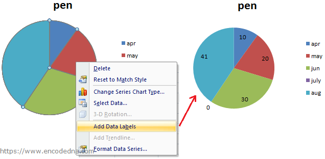
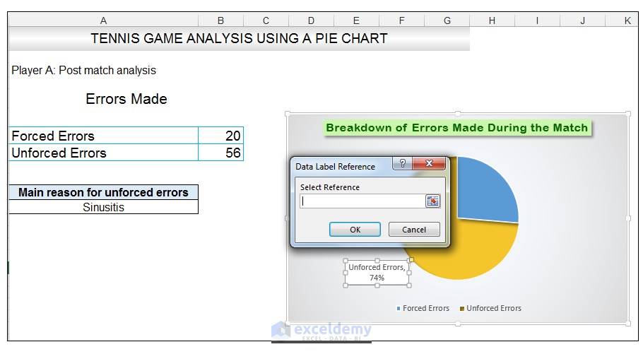
Possible to add second data label to pie chart? Re: Possible to add second data label to pie chart? Create the composite label in a worksheet column by concatenating the data in other cells and the nextline character, CHR (10). Now, use this composite label column as the source for Rob Bovey's add-in. -- Regards, Tushar Mehta Excel, PowerPoint, and VBA add-ins, tutorials How to Use Cell Values for Excel Chart Labels Select the chart, choose the "Chart Elements" option, click the "Data Labels" arrow, and then "More Options.". Uncheck the "Value" box and check the "Value From Cells" box. Select cells C2:C6 to use for the data label range and then click the "OK" button. The values from these cells are now used for the chart data labels. Excel Pie Chart Multiple Series - TheRescipes.info Creating Pie of Pie Chart in Excel: Follow the below steps to create a Pie of Pie chart: 1. In Excel, Click on the Insert tab. 2. In Excel, Click on the Insert tab. 2. Click on the drop-down menu of the pie chart from the list of the chart s. How to add or move data labels in Excel chart? To add or move data labels in a chart, you can do as below steps: In Excel 2013 or 2016. 1. Click the chart to show the Chart Elements button . 2. Then click the Chart Elements, and check Data Labels, then you can click the arrow to choose an option about the data labels in the sub menu. See screenshot: In Excel 2010 or 2007. 1. click on the ...

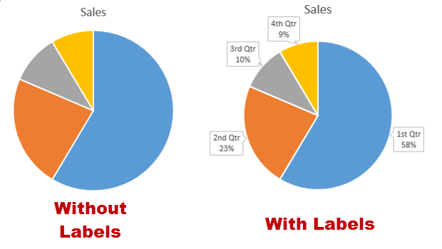
How to display leader lines in pie chart in Excel? To display leader lines in pie chart, you just need to check an option then drag the labels out. 1. Click at the chart, and right click to select Format Data Labels from context menu. 2. In the popping Format Data Labels dialog/pane, check Show Leader Lines in the Label Options section. See screenshot: 3. How to show percentage in pie chart in Excel? Please do as follows to create a pie chart and show percentage in the pie slices. 1. Select the data you will create a pie chart based on, click Insert > I nsert Pie or Doughnut Chart > Pie. See screenshot: 2. Then a pie chart is created. Right click the pie chart and select Add Data Labels from the context menu. 3. Pie Chart in Excel | How to Create Pie Chart | Step-by ... Step 1: Do not select the data; rather, place a cursor outside the data and insert one PIE CHART. Go to the Insert tab and click on a PIE. Step 2: once you click on a 2-D Pie chart, it will insert the blank chart as shown in the below image. Step 3: Right-click on the chart and choose Select Data. How to add data labels from different column in an Excel ... Right click the data series in the chart, and select Add Data Labels > Add Data Labels from the context menu to add data labels. 2. Click any data label to select all data labels, and then click the specified data label to select it only in the chart. 3.

How to Make a Pie Chart in Excel & Add Rich Data Labels to The Chart!

Adding data labels to a pie chart - Excel General - OzGrid ... Re: Adding data labels to a pie chart. Thanks again, norie. Really appreciate the help. I tried recording a macro while doing it manually (before my first post). But it didn't record anything about labels, much less making them bold.

How to Create a Pie Chart in Excel using Worksheet Data

How to Create Multi-Category Charts in Excel ... Step 1: Insert the data into the cells in Excel. Now select all the data by dragging and then go to "Insert" and select "Insert Column or Bar Chart". A pop-down menu having 2-D and 3-D bars will occur and select "vertical bar" from it. Select the cell -> Insert -> Chart Groups -> 2-D Column Bar Chart Insertion Multi-Category Chart

32 How To Label Vertical Axis In Excel - Labels Database 2020

Excel Pie Chart Data Table - TheRescipes.info Add Data Labels to the Pie Chart . There are many different parts to a chart in Excel, such as the plot area that contains the pie chart representing the selected data series, the legend, and the chart title and labels.

Excel & Google Sheets Chart Resources That Will Make Your Life Easier | PPC Hero

A Step-By-Step Guide on How to Make a Pie Chart in Excel ... A pie chart provides a visual representation of data sets in an Excel worksheet. Pie charts help define data sets with values that add up to form a whole. The pie chart looks like a pie or a doughnut, representing the different data entries as a percentage of a total in proportional slices.

Office: Display Data Labels in a Pie Chart

How to Combine or Group Pie Charts in Microsoft Excel Click on the first chart and then hold the Ctrl key as you click on each of the other charts to select them all. Click Format > Group > Group. All pie charts are now combined as one figure. They will move and resize as one image. Choose Different Charts to View your Data

How to Make a Pie Chart in Excel & Add Rich Data Labels to The Chart!

Datalabels formatter - animadigomma.it ShowValue ), the series name ( DataLabelBase First add data labels to the chart (Layout Ribbon > Data Labels) Define the new data label values in a bunch of cells, like this: Now, click on any data label. properties and restart the server: com. jaspersoft. md doc table datalabels 플러그인을 세팅하면 그래프 안에 수치가 주욱 ...

How to Make a Pie Chart in Excel & Add Rich Data Labels to The Chart!

How to Create a Pie Chart in Excel - Smartsheet To create a pie chart in Excel 2016, add your data set to a worksheet and highlight it. Then click the Insert tab, and click the dropdown menu next to the image of a pie chart. Select the chart type you want to use and the chosen chart will appear on the worksheet with the data you selected.

| Pryor Learning Solutions

Click the icon in the content placeholder that will allow ... Go to Normal View (click the Normal button on the bottom right) and display Excel allows you to add chart elements —including chart titles, legends, and data labels —to make your chart easier to read. 3 - Click Download Visual. Use the Selection pane to manage objects in your document: re-order them, show or hide them, and group or ungroup ...

Charts In Excel – Excel Tutorial World

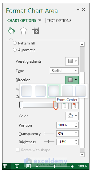
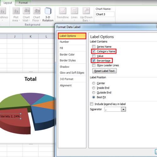
Change the format of data labels in a chart To get there, after adding your data labels, select the data label to format, and then click Chart Elements > Data Labels > More Options. To go to the appropriate area, click one of the four icons ( Fill & Line, Effects, Size & Properties ( Layout & Properties in Outlook or Word), or Label Options) shown here.

34 How To Label A Pie Chart - Labels Database 2020

Edit titles or data labels in a chart - support.microsoft.com On a chart, click one time or two times on the data label that you want to link to a corresponding worksheet cell. The first click selects the data labels for the whole data series, and the second click selects the individual data label. Right-click the data label, and then click Format Data Label or Format Data Labels.

34 Label Chart In Excel - Labels Database 2020

How to Create Pie Charts in Excel (In Easy Steps) 6. Create the pie chart (repeat steps 2-3). 7. Click the legend at the bottom and press Delete. 8. Select the pie chart. 9. Click the + button on the right side of the chart and click the check box next to Data Labels. 10. Click the paintbrush icon on the right side of the chart and change the color scheme of the pie chart. Result: 11.

Create A Pie Chart In Excel With and Easy Step-By-Step Guide

Pie of Pie Chart in Excel - Inserting, Customizing - Excel ... To add the data labels:- Select the chart and click on + icon at the top right corner of chart. Mark the check box containing data labels. Formatting Data Labels Consequently, this is going to insert default data labels on the chart.