42 row labels in excel pivot table
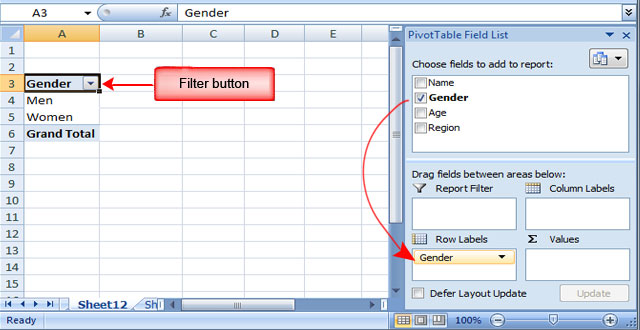
Sorting to your Pivot table row labels in custom order [quick tip] Using MATCH formula, find the order of each row label (in our case, classification) in the sort order list. Assuming classification is in D3, use =MATCH (D3, $I$3:$I$12, 0) Create a pivot table with data set including sort order column. Add sort order column along with classification to the pivot table row labels area. Pivot table row labels side by side - Excel Tutorials - OfficeTuts Excel You can copy the following table and paste it into your worksheet as Match Destination Formatting. Now, let's create a pivot table ( Insert >> Tables >> Pivot Table) and check all the values in Pivot Table Fields. Fields should look like this. Right-click inside a pivot table and choose PivotTable Options…. Check data as shown on the image below.
get a row label from pivot table - Microsoft Tech Community Creating PivotTable add data to data model by checking Create PivotTable and after that convert it to cube formulas. Now you may take these formulas and convert it to form you need, for example in H3 it could be =CUBEVALUE( "ThisWorkbookDataModel", CUBEMEMBER("ThisWorkbookDataModel", " [Measures].
Row labels in excel pivot table
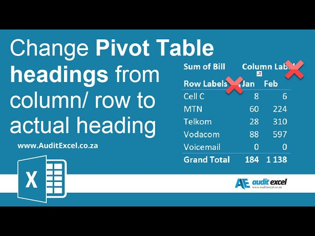
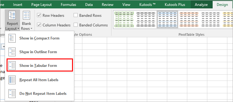
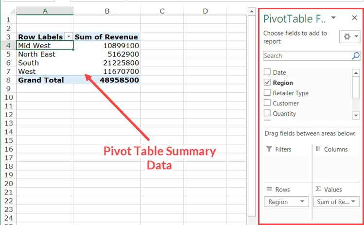
Pivot table row labels in separate columns • AuditExcel.co.za So when you click in the Pivot Table and click on the DESIGN tab one of the options is the Report Layout. Click on this and change it to Tabular form. Your pivot table report will now look like the bottom picture and will be easier to use in other areas of the spreadsheet and in our opinion is also easier to read. How to Group Data in Pivot Table (3 Simple Methods) Step 01: Insert a Pivot Table Firstly, select the dataset as shown below and click on the Insert ribbon. Then, you'll find the PivotTable drop-down on the right where you need to select the From Table/Range option. Next, a dialog box appears in which you have to check the New Worksheet option and press OK. Step 02: Construct Pivot Table Pivot Table "Row Labels" Header Frustration Pivot Table "Row Labels" Header Frustration. Hi Everyone please help I can't change my headers from Row Labels in a Pivot Table. Using Excel 365. Labels:
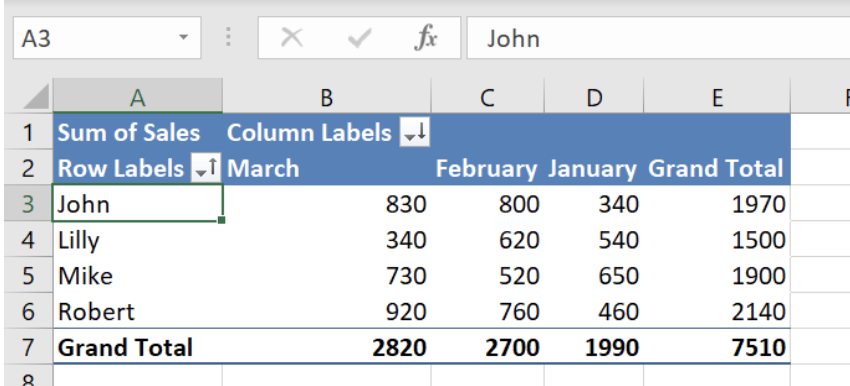
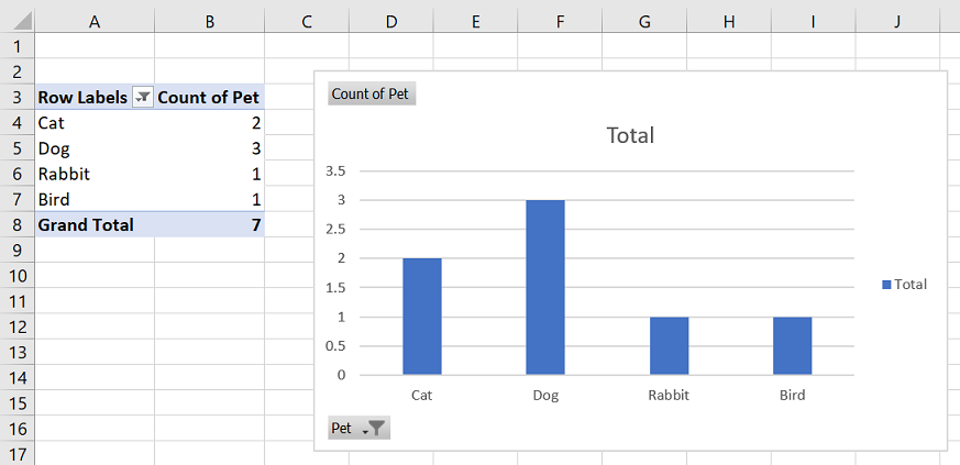
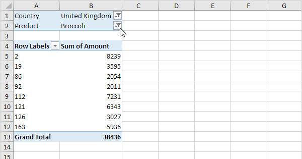
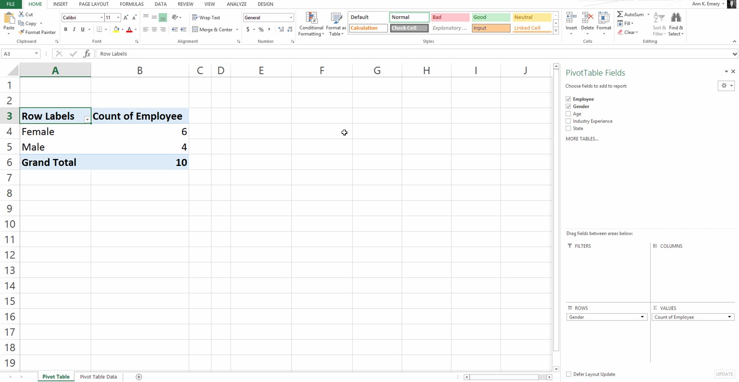
Row labels in excel pivot table. Match 2 columns, then return the sums : r/excel Hi Excel Reddit! I would like to create a formula that says if "Row Labels" matches the "Row labels" in the next table, the SUM "Votes" and "People" for both tables. How can this be done? Basically, if "AA" in the first table is also located in the next table, then sum "Votes" and "People" for both tables. Thank you! How to Flatten Data in Excel Pivot Table? - GeeksforGeeks Select a range that you want to flatten - typically, a column of labels. Highlight the empty cells only - hit F5 (GoTo) and select Special > Blanks. Type equals (=) and then the Up Arrow to enter a formula with a direct cell reference to the first data label. Instead of hitting enter, hold down Control and hit Enter. Data Model - Pivot - New Rows in Table | MrExcel Message Board The pivot table data source is the whole data table (not a range or anything like that). Later, I paste new rows of data to the bottom of the original data table, which become new lines of that table. The newly pasted rows of data show up in the pivot table. (upon refresh) Excel tutorial: How to filter a pivot table by rows or columns When you add a field as a row or column label in a pivot table, you automatically get the ability to filter the results in the table by items that appear in that field. Let's take a look. This pivot table is displaying just one field: Total Sales. After we add Product as a row label, notice that a drop-down arrow appears in the header area.
How to make row labels on same line in pivot table? - ExtendOffice In Excel, when you create a pivot table, the row labels are displayed as a compact layout, all the headings are listed in one column. Sometimes, you need to convert the compact layout to outline form to make the table more clearly. This article will tell you how to repeat row labels for group in Excel PivotTable. Multiple row labels on one row in Pivot table - MrExcel Message Board Try right clicking on the pivot table, over the labels, then choose Field Settings, on the Layout & Print tab, check the option to Show item labels in tabular form. M mssbass Active Member Joined Nov 14, 2002 Messages 252 Platform Windows Sep 28, 2012 #3 Unfortunately, changing this option did not change anything. PivotTable Count of Row Labels - Excel Help Forum Re: PivotTable Count of Row Labels. Please choose "Index" Option under the Pivot Table field options. Right Click on the field - "Value Field Settings" - "Show Value As" - chose "Index". Register To Reply. 05-15-2014, 12:17 PM #8. Move Row Labels in Pivot Table - Excel Pivot Tables Move Row Labels in Pivot Table. When you add fields to the row labels area in a pivot table, the field's items are automatically sorted. See how you can manually move those labels, to put them in a different order. There's a video and written steps below. In the screen shot below, the districts are listed alphabetically, from Central to West.
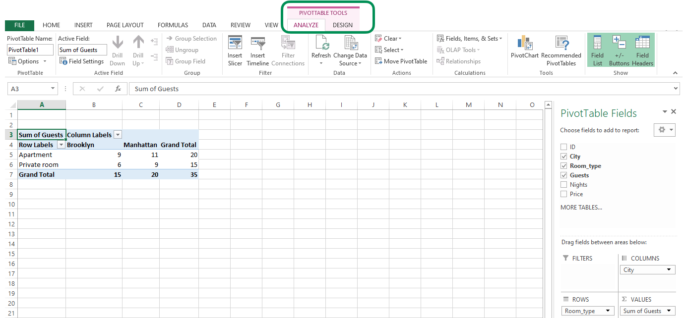
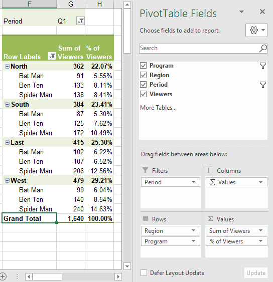
Multi-row and Multi-column Pivot Table - Excel Start Once the pivot table sheet is created, just like in the previous example, drag the Category and the Product to the Rows section and the Sales Value to the Values section to get the same Multi-Row pivot table we did in the previous example. Next we want to add a column. We will add the Date to the Column section by dragging the field. Remove row labels from pivot table • AuditExcel.co.za Click on the Pivot table. Click on the Design tab. Click on the report layout button. Choose either the Outline Format or the Tabular format. If you like the Compact Form but want to remove 'row labels' from the Pivot Table you can also achieve it by. Clicking on the Pivot Table. Clicking on the Analyse tab. How to Group Rows in Excel Pivot Table (3 Ways) - ExcelDemy Now select any number in the Row Labels of the table. Then right-click and select Group as shown below. Then, enter the Starting ( 60) and Ending ( 100) numbers and the difference ( 10) by which you want to group them. Next, hit OK. Finally, you will see the numbers grouped together as shown in the picture below.👇. Data Labels in Excel Pivot Chart (Detailed Analysis) 7 Suitable Examples with Data Labels in Excel Pivot Chart Considering All Factors 1. Adding Data Labels in Pivot Chart 2. Set Cell Values as Data Labels 3. Showing Percentages as Data Labels 4. Changing Appearance of Pivot Chart Labels 5. Changing Background of Data Labels 6. Dynamic Pivot Chart Data Labels with Slicers 7.
How to Sort Data in a Pivot Table | Excelchat
How do I fix row labels in pivot table? - vanjava.norushcharge.com To show the item labels in every row, for a specific pivot field: Right-click an item in the pivot field. In the Field Settings dialog box, click the Layout & Print tab.

Working with Pivot Tables | Excel library | Syncfusion
How to make row labels on same line in pivot table? - ExtendOffice Click any cell in your pivot table, and the PivotTable Tools tab will be displayed. 2. Under the PivotTable Tools tab, click Design > Report Layout > Show in Tabular Form, see screenshot: 3. And now, the row labels in the pivot table have been placed side by side at once, see screenshot: Group PivotTable Data by Sepcial Time
Lesson 54: Pivot Table Row Labels - Swotster
Change the pivot table "Row Labels" text | MrExcel Message Board 144. Feb 4, 2021. #3. mart37 said: Click on the cell and typ the text. Thanks mart37. So simple! I was looking for a way to change it on the ribbons & settings. Typical Excel - things you think are difficult are easy, and things that should be easy are difficult!

Repeat all item labels in Pivot Table (aka Fill in the blanks ...
Automatic Row And Column Pivot Table Labels - How To Excel At Excel Hit Pivot Table icon; Next select Pivot Table option; Select a table or range option; Select to put your Table on a New Worksheet or on the current one, for this tutorial select the first option; Click Ok; The Options and Design Tab will appear under the Pivot Table Tool; Select the check boxes next to the fields you want to use to add them to the Pivot Table

Pivot table row labels side by side – Excel Tutorials
Pivot Table Row Labels - Microsoft Community If you go to PivotTable Tools > Analyze > Layout > Report Layout > Show in Tabular Form, your column headers will be used for the row labels. Every once in a while there's a sudden gust of gravity... Report abuse 1 person found this reply helpful · Was this reply helpful? Yes No A. User Replied on December 19, 2017
Pivot Table headings that say column/ row instead of actual ...
Repeat item labels in a PivotTable - support.microsoft.com Right-click the row or column label you want to repeat, and click Field Settings. Click the Layout & Print tab, and check the Repeat item labels box. Make sure Show item labels in tabular form is selected. Notes: When you edit any of the repeated labels, the changes you make are applied to all other cells with the same label.
Rename Excel PivotTable headings - Office Watch
Design the layout and format of a PivotTable To change the layout of a PivotTable, you can change the PivotTable form and the way that fields, columns, rows, subtotals, empty cells and lines are displayed. To change the format of the PivotTable, you can apply a predefined style, banded rows, and conditional formatting. Windows Web Mac Changing the layout form of a PivotTable

pivot table row labels in separate columns 3 • AuditExcel.co.za
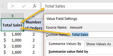
excel - Custom row labels in PivotTable - Stack Overflow 1 you can give nicknames to the fields that you are checking which populate the pivot table. If you go the pivot table data and right click you can change the value field settings to give a custom name to a row/series but I do not know about individual data points. path: pivot table data => right click => select Field Settings => edit custom name.

Repeat all item labels in Pivot Table (aka Fill in the blanks ...
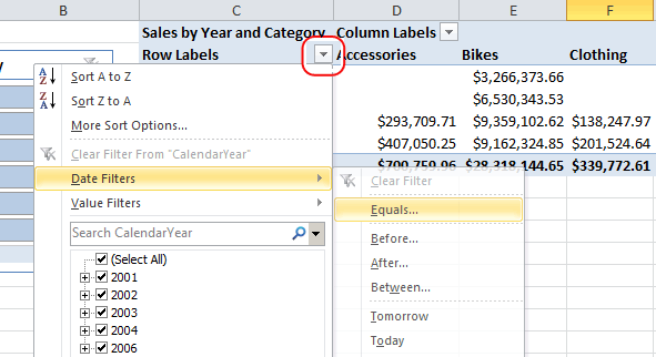
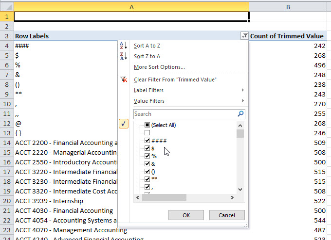
How to Use Excel Pivot Table Label Filters - Contextures Excel Tips To do that, you could click the drop down arrow for the Row or Column Labels, to see the list of pivot items in that pivot field. Then, in the list, remove the check mark for items you want to remove. For example, to hide the data for 7-Feb-10, you'd click on the check mark to remove it.
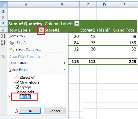
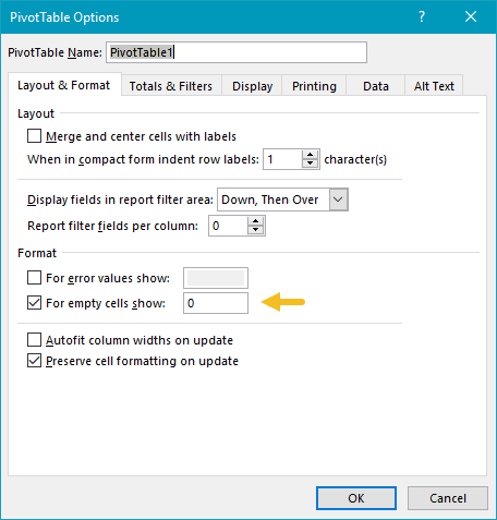
Excel 2016 – How to exclude (blank) values from pivot table
How to rename group or row labels in Excel PivotTable? - ExtendOffice To rename Row Labels, you need to go to the Active Field textbox. 1. Click at the PivotTable, then click Analyze tab and go to the Active Field textbox. 2. Now in the Active Field textbox, the active field name is displayed, you can change it in the textbox. You can change other Row Labels name by clicking the relative fields in the PivotTable, then rename it in the Active Field textbox.

Pivot table row labels in separate columns • AuditExcel.co.za
Pivot Table "Row Labels" Header Frustration Pivot Table "Row Labels" Header Frustration. Hi Everyone please help I can't change my headers from Row Labels in a Pivot Table. Using Excel 365. Labels:

Excel Pivot Tables: Insert Calculated Fields & Calculated ...
How to Group Data in Pivot Table (3 Simple Methods) Step 01: Insert a Pivot Table Firstly, select the dataset as shown below and click on the Insert ribbon. Then, you'll find the PivotTable drop-down on the right where you need to select the From Table/Range option. Next, a dialog box appears in which you have to check the New Worksheet option and press OK. Step 02: Construct Pivot Table
Excel Pivot Tables - Sorting Data
Pivot table row labels in separate columns • AuditExcel.co.za So when you click in the Pivot Table and click on the DESIGN tab one of the options is the Report Layout. Click on this and change it to Tabular form. Your pivot table report will now look like the bottom picture and will be easier to use in other areas of the spreadsheet and in our opinion is also easier to read.

Changing Order of Row Labels in Pivot Table

Pivot Tables Row Labels in Excel 2007 - YouTube

Pivot Table column label from horizontal to vertical ...
Filter dates in a PivotTable or PivotChart
Design the layout and format of a PivotTable

Identifying the Pivot Table fields for each row (Excel ...
Instructions for Transposing Pivot Table Data | Excelchat
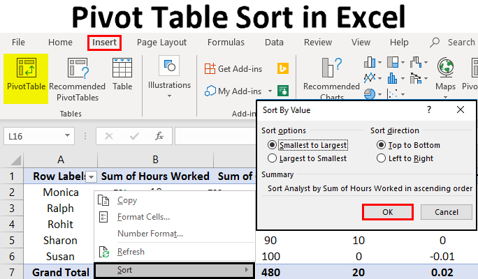
Pivot Table Sort in Excel | How to Sort Pivot Table Columns ...
Remove Blanks From Pivot Table Row Labels - Excel Dashboard ...

Excel pivot table shows only when rows have multiple other ...
How to Hide Blanks in Pivot Table

Excel pivot table shows only when rows have multiple other ...

Remove filter from ROW LABELS on pivot table Excel - Super User

Repeat Pivot Table row labels • AuditExcel.co.za Pivot Tables ...
Multi-level Pivot Table in Excel (In Easy Steps)
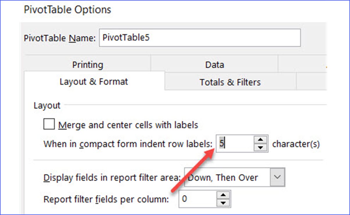
How to Increase Indent Row Labels in Pivot Table Compact Form ...
Manually Sorting Pivot Table Columns - Microsoft Tech Community
How to make row labels on same line in pivot table?
How to Delete a Pivot Table in Excel (Easy Step-by-Step Guide)

Repeat item labels in a PivotTable
The Pivot table tools ribbon in Excel
Pivot Table shows row labels instead of field name

Microsoft Excel – showing field names as headings rather than ...
Excel Pivot Tables Explained • My Online Training Hub

Change Pivot Table Sum of Headings and Blank Labels - YouTube
How to Save Time and Energy by Analyzing Your Data with Pivot ...

In pivot tables how can I replace Row Labels with field names ...

EXCEL: SETTING PIVOT TABLE DEFAULTS - Strategic Finance
Pivot Table: Pivot table display items with no data | Exceljet
Post a Comment for "42 row labels in excel pivot table"